Some Bayesian Finger-Puzzle Exercises, or: Often Wrong, Never In Doubt
Attention conservation notice: Clearing out my drafts folder. 600+ words on some examples that I cut from a recent manuscript. Only of interest to (bored) statisticians.
The theme here is to construct some simple yet pointed examples where Bayesian inference goes wrong, though the data-generating processes are well-behaved, and the priors look harmless enough. In reality, however, there is no such thing as an prior without bias, and in these examples the bias is so strong that Bayesian learning reaches absurd conclusions.
Example 1
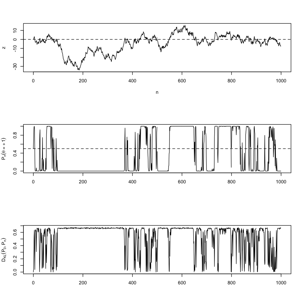
The data Xi, i=1,2,3,..., come from a 50/50 mixture of two Gaussians, with means at -1 and +1, both with standard deviation 1. (They are independent and identically distributed.) The prior, by coincidence, is a 50/50 mix of two Gaussians, located at -1 and +1, both with standard deviation 1. So initially the posterior predictive distribution coincides exactly with the actual data-generating distribution. After n observations x1, ... xn, whose sum is z, the log-likelihood ratio L(+1)/L(-1) is e2z. Hence the posterior probability that the expectation is +1 is 1/(1+e-2z), and the posterior probability that the expectation is -1 is 1/(1+e2z). The sufficient statistic z itself follows an unbiased random walk, meaning that as n grows it tends to get further and further away from the origin, with a typical size growing roughly like n1/2. It does keep returning to the origin, at intervals dictated by the arc sine law, but it spends more and more of its time very far away from it. The posterior estimate of the mean thus wanders from being close to +1 to being close to -1 and back erratically, hardly ever spending time near zero, even though (from the law of large numbers) the sample mean converges to zero.
This figure shows typical sample paths for z, for the posterior probability of the +1 mode, and for the relative entropy of the predictive distribution from the data-generating distribution. (The latter is calculated by Monte Carlo since I've forgotten how to integrate, so some of the fuzziness is MC noise.) Here is the R code.

Exercise 1: Confirm those calculations for the likelihood ratio and so for the posterior.
Exercise 2: Find the expected log-likelihood of an arbitrary-mean unit-variance Gaussian under this data-generating distribution.
Example 2
Keep the same data-generating distribution, but now let the prior be the conjugate prior for a Gaussian, namely another Gaussian, centered at zero. The posterior is then another Gaussian, which is a function of the sample mean, since the latter is a sufficient statistic for the problem.
Exercise 3: Find the mean and variance of the posterior distribution as functions of the sample mean. (You could look them up, but that would be cheating.)
As we get more and more data, the sample mean of converges almost surely to zero (by the law of large numbers), which here drives the mean and variance of the posterior to zero almost surely as well. In other words, the Bayesian becomes dogmatically certain that the data are distributed according to a standard Gaussian with mean 0 and variance 1. This is so even though the sample variance almost surely converges to the true variance, which is 2. This Bayesian, then, is certain that the data are really not that variable, and any time now will start settling down.
Exercise 4: Suppose that we take the prior from the previous example, set it to 0 on the interval [-1,+1], and increase the prior everywhere else by a constant factor to keep it normalized. Show that the posterior density at every point except -1 and +1 will go to zero. (Hint: use exercise 2 and see here.)
Update in response to e-mails, 27 March: No, I'm not saying that actual Bayesian statisticians are this dumb. A sensible practitioner would, as Andy Gelman always recommends, run a posterior predictive check, and discover that his estimated model looks nothing at all like the data. But that sort of thing is completely outside the formal apparatus of Bayesian inference. What amuses me in these examples is that the formal machinery becomes so certain while being so wrong, while starting from the right answer (and this while Theorem 5 from my paper still applies!). See the second post by Brad DeLong, linked to below.
Manual trackback: Brad DeLong; and again Brad DeLong (with a simpler version of example 1!); The Statistical Mechanic
Posted at March 26, 2009 10:45 | permanent link