Speaking Truth to Power About Weblogs, or, How Not to Draw a Straight Line
Now that Henry Farrell and Dan Drezner's paper on political weblogs is launched on the world, it may amuse some of you to read about some of the behind-the-scenes details. I have tried to explain what power laws are, and why physicists care about them so much, over in my notebooks, and I won't repeat myself here.
My involvement began in April, when Henry asked me some questions about how to estimate the exponent of a power law. This evoked from me a long rant about how not to do it, which I ended by offering to do the analysis myself, partly out of guilt at subjecting the poor man to my ravings, and partly as a way of practicing my R skills. Henry, who has a grossly (if flatteringly) exaggerated opinion of my expertise, took me up on the offer.
The first thing I did was to discard part of the data. Power-law distributions, like many other distributions with heavy tails, are only defined over positive values, and there were a lot of blogs which had no incoming links. I don't feel bad about that, because in a sense they're not really part of the network. Then I calculated, for each in-degree d, the fraction of blogs whose in-degree was greater than or equal to d.
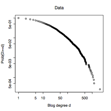
Notice that this curve is definitely curved, and in fact concave --- if you pick any two points on it, and draw their cord, or straight line connecting them, the curve lives above the cord. If, nonetheless, I do the usual least-squares straight-line fit, I get the line in the next picture, with a slope of -1.15. The R^2 was 0.898, which is to say, the fitted line accounts for 89.8 percent of the variance in the figure. (I'm only reporting numbers to three significant figures.) This is, I dare say, good enough for Physica A.
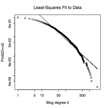
This procedure --- find your power-law distribution by linear regression, and verify that it is a power law by finding a high R^2 --- is a very common one in the statistical physics/complex systems literature. It suffers from two problems. (1) It does not produce a power-law distribution. (2) It does not reliably distinguish between power laws and other distributions.
As to (1), the problem is that nothing in the usual procedure ensures that the line you fit meets the y-axis at 1. That means that the total probability doesn't add up to 1, and the curve isn't really a probability distribution at all; end of story. However, if your data comes from a Pareto distribution, then the log-log slope constitutes a consistent estimate of the exponent. Even then, however, you are better off estimating the parameters of the distribution using maximum likelihood (as I do below).
As to (2), the simple fact is that any smooth curve looks like a straight line, if you look at a small enough piece of it. (More exactly, any differentiable function can be approximated arbitrarily well by a linear function over a sufficiently small range; that's what it means to be differentiable. If you're looking at a probability distribution, having a derivative means that the probability density exists.) And this range can extend over multiple orders of magnitude.
Here's an example to back that up. I took a log-normal probability distribution, with a mean log of 0 and a standard deviation in the log of 3, and drew ten thousand random numbers from it. This sample gave me the following empirical probability distribution.

Then I just took the sub-sample where the random numbers were greater than or equal to 1, and did a least-squares fit to them.
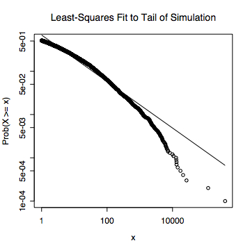
That line is the result of fitting to 5112 points, extending over four orders of magnitude. It has an R^2 of 0.962. Clearly, R^2 has next to no power to detect departures from a power-law. Even if I cheated, and gave the regression the exact log-normal probability of every integer point over the range of that plot, things wouldn't be any better; in fact I'd then get an R^2 of 0.994!
(As an aside, if you find a paper which reports error bars on the slope based on a least-squares fit --- that would be ± 0.022 for the data --- you can throw it away. The usual procedure for calculating margins of error in linear regression assumes that the fluctuations of observed values around their means have a Gaussian distribution. Here, this would mean that the log of the relative frequency equals the log of probability, plus Gaussian noise. But, if you assume that these are independent samples, and you have enough of them to do sensible statistics, then the central limit theorem says that the relative frequency equals the probability plus Gaussian noise, and this is incompatible with the same relationship holding between their logarithms.)
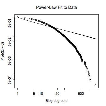
Having discarded linear regression, I do a maximum likelihood fit to the discrete Pareto distribution. Curiously enough, this distribution does not have a standard implementation in R. Formally, the probability mass function is $ P(D=d) = d^{-\alpha}/\zeta(\alpha) $, where $ \zeta(\alpha) $ is the normalizing factor or partition function required to make the probabilities sum to 1. I've written it $ \zeta(\alpha) $ for two reasons: first, physicists traditionally write $Z$ or $z$ for the partition function, and second, it happens to be the Riemann zeta function famous from number theory, Cryptonomicon, etc., $ \zeta(\alpha) = \sum_{k=1}^{\infty}{k^{-\alpha}} $. The log-likelihood function is $ L(\alpha) = -\alpha \sum_{i=1}^{n}{d_i} - \log{\zeta(\alpha)} $, where $ d_i $ is the degree of weblog number $i$. We want to find the $ \alpha $ which maximizes $ L(\alpha) $. Fortunately, R has a rather good nonlinear maximization routine built in, so I just turned it over to that, once I'd taught it how to calculate the zeta function. The result was an exponent of $-1.30 \pm 0.006$. (The calculation of the standard error is based on asymptotic formulas, so I'm a bit skeptical of it, but not sufficiently motivated to do better.) It plots out as follows.
Now I turn to my main alternative, the most boring possible rival to the power-law within the field of heavy-tailed distributions, namely, the log-normal. Just as the Gaussian distribution is the limit of what you get by summing up many independent quantities, the log-normal is the limit of multiplying independent quantities. I won't repeat the log-likelihood calculation, and just say that it gives me the following curve (mean of log $2.60 \pm 0.02$, standard deviation of log $1.48 \pm 0.02$).

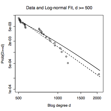
Next, I take a closer look at the tail --- say, somewhat arbitrarily, blogs with an in-degree of 500 or more. (Changing the threshold makes little difference.) In the next figure, the log-normal fit to the complete data is the straight line, and the linear regression on the points in the tail is the dashed line. Notice that the log-normal fit is still quite good, and that the log-normal line looks quite straight --- you can just see a bit of curvature if you squint.
At this point, to be really rigorous, I should do some kind of formal test to compare the two hypotheses. What I should really calculate, following the general logic of error statistics, is the probability of getting that good of a fit to a log-normal if the data really came from a power law, and vice versa. But just look at the curves!

A bit more quantitatively, the log-likelihoods were -18481.51 for the power-law and -17218.22 for the log-normal. This means that the observed data were about 13 million times more likely under a log-normal than under the best-fitting power law. In a case like this, under any non-insane test, the power law loses.
Update, 28 November 2007: Modesty forbids me to recommend that you read our paper about power law inference in place of others, but I am not a modest man. (The analysis of this data didn't make that paper, simply for reasons of length.)
Update, 28 June 2010: Some ideas are zombies.
Manual trackback: Science after Sunclipse
Posted at August 08, 2004 09:40 | permanent link